dask.delayed - parallelize any code

You can run this notebook in a live session or view it on Github.

$Dask logo\$

dask.delayed - parallelize any code¶

What if you don’t have an array or dataframe? Instead of having blocks where the function is applied to each block, you can decorate functions with @delayed and have the functions themselves be lazy.

This is a simple way to use dask to parallelize existing codebases or build complex systems.

Related Documentation

As we’ll see in the distributed scheduler notebook, Dask has several ways of executing code in parallel. We’ll use the distributed scheduler by creating a dask.distributed.Client. For now, this will provide us with some nice diagnostics. We’ll talk about schedulers in depth later.

[1]:

from dask.distributed import Client

client = Client(n_workers=4)

A Typical Workflow¶

Typically if a workflow contains a for-loop it can benefit from delayed. The following example outlines a read-transform-write:

import dask

@dask.delayed
def process_file(filename):
    data = read_a_file(filename)
    data = do_a_transformation(data)
    destination = f"results/{filename}"
    write_out_data(data, destination)
    return destination

results = []
for filename in filenames:
    results.append(process_file(filename))

dask.compute(results)

Basics¶

First let’s make some toy functions, inc and add, that sleep for a while to simulate work. We’ll then time running these functions normally.

In the next section we’ll parallelize this code.

[2]:

from time import sleep


def inc(x):
    sleep(1)
    return x + 1


def add(x, y):
    sleep(1)
    return x + y

We time the execution of this normal code using the %%time magic, which is a special function of the Jupyter Notebook.

[3]:

%%time
# This takes three seconds to run because we call each
# function sequentially, one after the other

x = inc(1)
y = inc(2)
z = add(x, y)

CPU times: user 107 ms, sys: 26 ms, total: 133 ms
Wall time: 3 s

Parallelize with the `dask.delayed` decorator¶

Those two increment calls could be called in parallel, because they are totally independent of one-another.

We’ll make the inc and add functions lazy using the dask.delayed decorator. When we call the delayed version by passing the arguments, exactly as before, the original function isn’t actually called yet - which is why the cell execution finishes very quickly. Instead, a delayed object is made, which keeps track of the function to call and the arguments to pass to it.

[4]:

import dask


@dask.delayed
def inc(x):
    sleep(1)
    return x + 1


@dask.delayed
def add(x, y):
    sleep(1)
    return x + y

[5]:

%%time
# This runs immediately, all it does is build a graph

x = inc(1)
y = inc(2)
z = add(x, y)

CPU times: user 241 µs, sys: 43 µs, total: 284 µs
Wall time: 273 µs

This ran immediately, since nothing has really happened yet.

To get the result, call compute. Notice that this runs faster than the original code.

[6]:

%%time
# This actually runs our computation using a local thread pool

z.compute()

CPU times: user 186 ms, sys: 35.8 ms, total: 222 ms
Wall time: 2.14 s

[6]:

What just happened?¶

The z object is a lazy Delayed object. This object holds everything we need to compute the final result, including references to all of the functions that are required and their inputs and relationship to one-another. We can evaluate the result with .compute() as above or we can visualize the task graph for this value with .visualize().

[7]:

[7]:

Delayed('add-3602d5e7-31dd-4b69-a059-cabe0549954f')

[8]:

# Look at the task graph for `z`
z.visualize()

[8]:

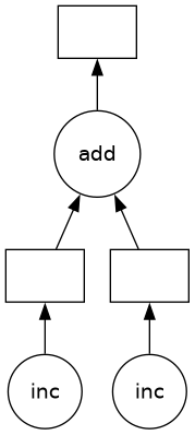
Notice that this includes the names of the functions from before, and the logical flow of the outputs of the inc functions to the inputs of add.

Some questions to consider:¶

Why did we go from 3s to 2s? Why weren’t we able to parallelize down to 1s?
What would have happened if the inc and add functions didn’t include the sleep(1)? Would Dask still be able to speed up this code?
What if we have multiple outputs or also want to get access to x or y?

Exercise: Parallelize a for loop¶

for loops are one of the most common things that we want to parallelize. Use dask.delayed on inc and sum to parallelize the computation below:

[9]:

data = [1, 2, 3, 4, 5, 6, 7, 8]

[10]:

%%time
# Sequential code


def inc(x):
    sleep(1)
    return x + 1


results = []
for x in data:
    y = inc(x)
    results.append(y)

total = sum(results)

CPU times: user 261 ms, sys: 76.9 ms, total: 338 ms
Wall time: 8.01 s

[11]:

total

[11]:

[12]:

%%time
# Your parallel code here...

CPU times: user 3 µs, sys: 1e+03 ns, total: 4 µs
Wall time: 5.72 µs

[13]:

@dask.delayed
def inc(x):
    sleep(1)
    return x + 1


results = []
for x in data:
    y = inc(x)
    results.append(y)

total = sum(results)
print("Before computing:", total)  # Let's see what type of thing total is
result = total.compute()
print("After computing :", result)  # After it's computed

Before computing: Delayed('add-f563d63b41f91fd63da9dec08e1dcb34')
After computing : 44

How do the graph visualizations compare with the given solution, compared to a version with the sum function used directly rather than wrapped with delayed? Can you explain the latter version? You might find the result of the following expression illuminating

inc(1) + inc(2)

Exercise: Parallelize a for-loop code with control flow¶

Often we want to delay only some functions, running a few of them immediately. This is especially helpful when those functions are fast and help us to determine what other slower functions we should call. This decision, to delay or not to delay, is usually where we need to be thoughtful when using dask.delayed.

In the example below we iterate through a list of inputs. If that input is even then we want to call inc. If the input is odd then we want to call double. This is_even decision to call inc or double has to be made immediately (not lazily) in order for our graph-building Python code to proceed.

[14]:

def double(x):
    sleep(1)
    return 2 * x


def is_even(x):
    return not x % 2


data = [1, 2, 3, 4, 5, 6, 7, 8, 9, 10]

[15]:

%%time
# Sequential code

results = []
for x in data:
    if is_even(x):
        y = double(x)
    else:
        y = inc(x)
    results.append(y)

total = sum(results)
print(total)

Delayed('add-be32c1dc62a029f9d9b1a55e0be45350')
CPU times: user 183 ms, sys: 32.3 ms, total: 216 ms
Wall time: 5.01 s

[16]:

%%time
# Your parallel code here...
# TODO: parallelize the sequential code above using dask.delayed
# You will need to delay some functions, but not all

CPU times: user 2 µs, sys: 0 ns, total: 2 µs
Wall time: 5.48 µs

[17]:

@dask.delayed
def double(x):
    sleep(1)
    return 2 * x


results = []
for x in data:
    if is_even(x):  # even
        y = double(x)
    else:  # odd
        y = inc(x)
    results.append(y)

total = sum(results)

[18]:

%time total.compute()

CPU times: user 144 ms, sys: 14.9 ms, total: 159 ms
Wall time: 3.04 s

[18]:

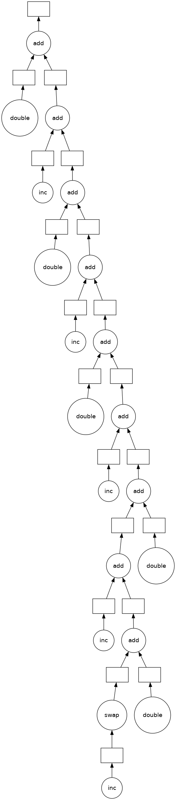
[19]:

total.visualize()

[19]:

Some questions to consider:¶

What are other examples of control flow where we can’t use delayed?
What would have happened if we had delayed the evaluation of is_even(x) in the example above?
What are your thoughts on delaying sum? This function is both computational but also fast to run.

Exercise: Parallelize a Pandas Groupby Reduction¶

In this exercise we read several CSV files and perform a groupby operation in parallel. We are given sequential code to do this and parallelize it with dask.delayed.

The computation we will parallelize is to compute the mean departure delay per airport from some historical flight data. We will do this by using dask.delayed together with pandas. In a future section we will do this same exercise with dask.dataframe.

Create data¶

Run this code to prep some data.

This downloads and extracts some historical flight data for flights out of NYC between 1990 and 2000. The data is originally from here.

[20]:

%run prep.py -d flights

Inspect data¶

[21]:

import os

sorted(os.listdir(os.path.join("data", "nycflights")))

[21]:

['1990.csv',
 '1991.csv',
 '1992.csv',
 '1993.csv',
 '1994.csv',
 '1995.csv',
 '1996.csv',
 '1997.csv',
 '1998.csv',
 '1999.csv']

Read one file with `pandas.read_csv` and compute mean departure delay¶

[22]:

import pandas as pd

df = pd.read_csv(os.path.join("data", "nycflights", "1990.csv"))
df.head()

[22]:

	Year	Month	DayofMonth	DayOfWeek	DepTime	CRSDepTime	ArrTime	CRSArrTime	UniqueCarrier	FlightNum	...	AirTime	ArrDelay	DepDelay	Origin	Dest	Distance	TaxiIn	TaxiOut
0	1990	1	1	1	1621.0	1540	1747.0	1701	US	33	...	NaN	46.0	41.0	EWR	PIT	319.0	NaN	NaN
1	1990	1	2	2	1547.0	1540	1700.0	1701	US	33	...	NaN	-1.0	7.0	EWR	PIT	319.0	NaN	NaN
2	1990	1	3	3	1546.0	1540	1710.0	1701	US	33	...	NaN	9.0	6.0	EWR	PIT	319.0	NaN	NaN
3	1990	1	4	4	1542.0	1540	1710.0	1701	US	33	...	NaN	9.0	2.0	EWR	PIT	319.0	NaN	NaN
4	1990	1	5	5	1549.0	1540	1706.0	1701	US	33	...	NaN	5.0	9.0	EWR	PIT	319.0	NaN	NaN

5 rows × 23 columns

[23]:

# What is the schema?
df.dtypes

[23]:

Year                   int64
Month                  int64
DayofMonth             int64
DayOfWeek              int64
DepTime              float64
CRSDepTime             int64
ArrTime              float64
CRSArrTime             int64
UniqueCarrier         object
FlightNum              int64
TailNum              float64
ActualElapsedTime    float64
CRSElapsedTime         int64
AirTime              float64
ArrDelay             float64
DepDelay             float64
Origin                object
Dest                  object
Distance             float64
TaxiIn               float64
TaxiOut              float64
Cancelled              int64
Diverted               int64
dtype: object

[24]:

# What originating airports are in the data?
df.Origin.unique()

[24]:

array(['EWR', 'LGA', 'JFK'], dtype=object)

[25]:

# Mean departure delay per-airport for one year
df.groupby("Origin").DepDelay.mean()

[25]:

Origin
EWR    10.854962
JFK    17.027397
LGA    10.895592
Name: DepDelay, dtype: float64

Sequential code: Mean Departure Delay Per Airport¶

The above cell computes the mean departure delay per-airport for one year. Here we expand that to all years using a sequential for loop.

[26]:

from glob import glob

filenames = sorted(glob(os.path.join("data", "nycflights", "*.csv")))

[27]:

%%time

sums = []
counts = []
for fn in filenames:
    # Read in file
    df = pd.read_csv(fn)

    # Groupby origin airport
    by_origin = df.groupby("Origin")

    # Sum of all departure delays by origin
    total = by_origin.DepDelay.sum()

    # Number of flights by origin
    count = by_origin.DepDelay.count()

    # Save the intermediates
    sums.append(total)
    counts.append(count)

# Combine intermediates to get total mean-delay-per-origin
total_delays = sum(sums)
n_flights = sum(counts)
mean = total_delays / n_flights

CPU times: user 42.6 ms, sys: 9.62 ms, total: 52.2 ms
Wall time: 54.8 ms

[28]:

mean

[28]:

Origin
EWR    12.500968
JFK          NaN
LGA    10.169227
Name: DepDelay, dtype: float64

Parallelize the code above¶

Use dask.delayed to parallelize the code above. Some extra things you will need to know.

Methods and attribute access on delayed objects work automatically, so if you have a delayed object you can perform normal arithmetic, slicing, and method calls on it and it will produce the correct delayed calls.
Calling the .compute() method works well when you have a single output. When you have multiple outputs you might want to use the dask.compute function. This way Dask can share the intermediate values.

So your goal is to parallelize the code above (which has been copied below) using dask.delayed. You may also want to visualize a bit of the computation to see if you’re doing it correctly.

[29]:

%%time
# your code here

CPU times: user 2 µs, sys: 1 µs, total: 3 µs
Wall time: 5.96 µs

If you load the solution, add %%time to the top of the cell to measure the running time.

[30]:

%%time

# This is just one possible solution, there are
# several ways to do this using `dask.delayed`


@dask.delayed
def read_file(filename):
    # Read in file
    return pd.read_csv(filename)


sums = []
counts = []
for fn in filenames:
    # Delayed read in file
    df = read_file(fn)

    # Groupby origin airport
    by_origin = df.groupby("Origin")

    # Sum of all departure delays by origin
    total = by_origin.DepDelay.sum()

    # Number of flights by origin
    count = by_origin.DepDelay.count()

    # Save the intermediates
    sums.append(total)
    counts.append(count)

# Combine intermediates to get total mean-delay-per-origin
total_delays = sum(sums)
n_flights = sum(counts)
mean, *_ = dask.compute(total_delays / n_flights)

CPU times: user 104 ms, sys: 17.8 ms, total: 122 ms
Wall time: 804 ms

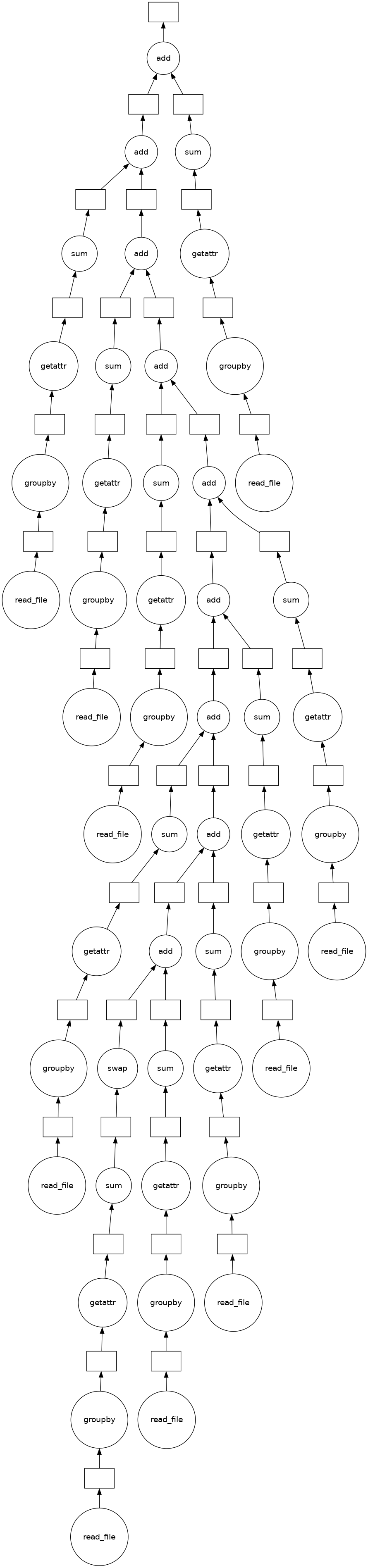
[31]:

(sum(sums)).visualize()

[31]:

[32]:

# ensure the results still match
mean

[32]:

Origin
EWR    12.500968
JFK          NaN
LGA    10.169227
Name: DepDelay, dtype: float64

Some questions to consider:¶

How much speedup did you get? Is this how much speedup you’d expect?
Experiment with where to call compute. What happens when you call it on sums and counts? What happens if you wait and call it on mean?
Experiment with delaying the call to sum. What does the graph look like if sum is delayed? What does the graph look like if it isn’t?
Can you think of any reason why you’d want to do the reduction one way over the other?

Learn More¶

Visit the Delayed documentation. In particular, this delayed screencast will reinforce the concepts you learned here and the delayed best practices document collects advice on using dask.delayed well.

Close the Client¶

Before moving on to the next exercise, make sure to close your client or stop this kernel.

[33]:

client.close()

Dask Arrays - parallelized numpy

Distributed - spread your data and computation across a cluster

Dask Tutorial documentation

dask.delayed - parallelize any code

Contents

dask.delayed - parallelize any code¶

A Typical Workflow¶

Basics¶

Parallelize with the `dask.delayed` decorator¶

What just happened?¶

Some questions to consider:¶

Exercise: Parallelize a for loop¶

Exercise: Parallelize a for-loop code with control flow¶

Some questions to consider:¶

Exercise: Parallelize a Pandas Groupby Reduction¶

Create data¶

Inspect data¶

Read one file with `pandas.read_csv` and compute mean departure delay¶

Sequential code: Mean Departure Delay Per Airport¶

Parallelize the code above¶

Some questions to consider:¶

Learn More¶

Close the Client¶

Dask Tutorial documentation

dask.delayed - parallelize any code

Contents

dask.delayed - parallelize any code¶

A Typical Workflow¶

Basics¶

Parallelize with the dask.delayed decorator¶

What just happened?¶

Some questions to consider:¶

Exercise: Parallelize a for loop¶

Exercise: Parallelize a for-loop code with control flow¶

Some questions to consider:¶

Exercise: Parallelize a Pandas Groupby Reduction¶

Create data¶

Inspect data¶

Read one file with pandas.read_csv and compute mean departure delay¶

Sequential code: Mean Departure Delay Per Airport¶

Parallelize the code above¶

Some questions to consider:¶

Learn More¶

Close the Client¶

Parallelize with the `dask.delayed` decorator¶

Read one file with `pandas.read_csv` and compute mean departure delay¶